Note
Go to the end to download the full example code.
Survival analysis with SurvivalBoost#
Survival analysis is a time-to-event regression problem that deals with censored data. We refer to individuals as censored if they did not experience the event during the period of observation.
In our setting, we are mostly interested in right-censored data, which means that the event of interest did not occur before the end of the observation period (typically the time of data collection).
We will use the The Molecular Taxonomy of Breast Cancer International Consortium
(METABRIC) dataset as an example, which is available through pycox.datasets. This
is the processed data set used in the
DeepSurv paper (Katzman et al. 2018).
import numpy as np
import pandas as pd

from pycox.datasets import metabric


np.random.seed(0)

df = metabric.read_df()
X = df.drop(columns=["event", "duration"])
y = df[["event", "duration"]]
y
Dataset 'metabric' not locally available. Downloading...
Done
Notice that the target y is comprised of two columns:
event, where \(0\) marks censoring and \(1\) is indicative that the event of interest (death) has actually happened before the end of the observation window.duration, the censored time-to-event \(D = \min(T, C) > 0\). This is the minimum between the date of the experienced event, represented by the random variable \(T\), and the censoring date, represented by \(C\).
In this dataset, approximately 42% of the data is censored..
y["event"].value_counts(normalize=True)
event
1    0.579307
0    0.420693
Name: proportion, dtype: float64
from sklearn.model_selection import train_test_split


X_train, X_test, y_train, y_test = train_test_split(X, y, test_size=0.3)
Using SurvivalBoost to estimate the survival function#
Here, our quantity of interest is the survival probability:
This represents the probability that an event doesn’t occur at or before some given time \(t\), i.e. that it happens at some time \(T > t\), given the patient features \(x\).
SurvivalBoost is a scikit-learn compatible model which expects a covariates dataframe
(or array-like) X, and a target dataframe y with columns “event” and
“duration”. This allows SurvivalBoost to estimate the survival function \(S\).
from hazardous import SurvivalBoost


survival_boost = SurvivalBoost(show_progressbar=False).fit(X_train, y_train)
survival_boost
/opt/hostedtoolcache/Python/3.10.16/x64/lib/python3.10/site-packages/sklearn/utils/deprecation.py:151: FutureWarning: 'force_all_finite' was renamed to 'ensure_all_finite' in 1.6 and will be removed in 1.8.
  warnings.warn(
SurvivalBoost can then predict the survival function for each patient,
according to some time grid of horizons.
The time grid is learned during fit but can be passed during prediction
with the parameter times.
When times is set to None, the model will used the learned time grid.
predicted_curves = survival_boost.predict_cumulative_incidence(
    X_test,
    times=None,
)

survival_curves = predicted_curves[:, 0]  # survival function S(t)
incidence_curves = predicted_curves[:, 1]  # cumulative incidence of the event (death)
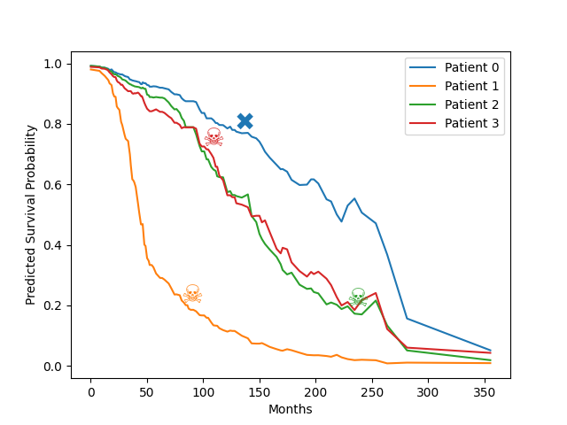
Let’s plot the estimated survival function for some patients.
import matplotlib.pyplot as plt


fig, ax = plt.subplots()

patient_ids_to_plot = [0, 1, 2, 3]

for idx in patient_ids_to_plot:
    ax.plot(survival_boost.time_grid_, survival_curves[idx], label=f"Patient {idx}")

    # plot symbols for death or censoring
    event = y_test.iloc[idx]["event"]
    duration = y_test.iloc[idx]["duration"]

    # find the index of time closest to duration
    jdx = np.searchsorted(survival_boost.time_grid_, duration)
    smiley = "☠️" if event == 1 else "✖"
    ax.text(
        duration,
        survival_curves[idx, jdx],
        smiley,
        fontsize=20,
        color=ax.lines[idx].get_color(),
    )

ax.legend()
ax.set_title("")
ax.set_xlabel("Months")
ax.set_ylabel("Predicted Survival Probability")

plt.show()

Measuring features impact on predictions#
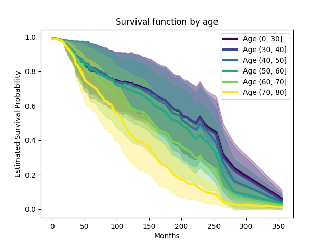
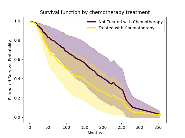
We can also observe the survival function by age group or by chemotherapy treatment to show the impact that the model attributes to these features. We do something akin to Partial Dependence Plots, where we sample the feature independently of the other features to eliminate correlations.
We create a synthetic dataset where age (x8) is resampled to reduce
confounder bias.
X_synthetic = X_train.copy()
# Age varies from 20 to 80
X_synthetic["x8"] = np.linspace(20, 80, X_synthetic.shape[0])

# Predict cumulative incidence on the synthetic dataset
survival_curves_synthetic = survival_boost.predict_survival_function(X_synthetic)

# Create age bins and sort them by the left bin edge
age_bins = pd.cut(X_synthetic["x8"], bins=[0, 30, 40, 50, 60, 70, 80, 90, 100])
age_groups = sorted(age_bins.unique(), key=lambda x: x.left)

# Create a colormap
fig, ax = plt.subplots()
cmap = plt.get_cmap("viridis", len(age_groups))

for idx, age_group in enumerate(age_groups):
    # Get the mask of patients in the current age group
    mask = age_bins == age_group

    # Calculate the mean and std cumulative incidence for the current age group
    mean_survival = survival_curves_synthetic[mask].mean(axis=0)
    std_survival = survival_curves_synthetic[mask].std(axis=0)

    # Plot with color from colormap
    ax.plot(
        survival_boost.time_grid_,
        mean_survival,
        label=f"Age {age_group}",
        color=cmap(idx),
        linewidth=3,
    )
    # Add ribbon for std
    ax.fill_between(
        survival_boost.time_grid_,
        mean_survival - std_survival,
        mean_survival + std_survival,
        color=cmap(idx),
        alpha=0.3,
    )

ax.legend()
ax.set_title("Survival function by age")
ax.set_xlabel("Months")
ax.set_ylabel("Estimated Survival Probability")

plt.show()

Unsurprisingly, the cumulative incidence of death mostly increases with age. We can do the same thing with chemotherapy treatement.
Let’s create a synthetic dataset where chemotherapy (x6)
alternates between 0 and 1.
X_synthetic = X_train.copy()
X_synthetic["x6"] = np.tile([0, 1], X_synthetic.shape[0] // 2)

survival_curves_synthetic = survival_boost.predict_survival_function(
    X_synthetic,
)

fig, ax = plt.subplots()
cmap = plt.get_cmap("viridis", 2)

for chemo_group in [0, 1]:
    mask = X_synthetic["x6"] == chemo_group
    mean_survival = survival_curves_synthetic[mask].mean(axis=0)
    std_survival = survival_curves_synthetic[mask].std(axis=0)
    ax.plot(
        survival_boost.time_grid_,
        mean_survival,
        label=(
            "Treated with Chemotherapy"
            if chemo_group == 1
            else "Not Treated with Chemotherapy"
        ),
        color=cmap(chemo_group),
        linewidth=3,
    )
    ax.fill_between(
        survival_boost.time_grid_,
        mean_survival - std_survival,
        mean_survival + std_survival,
        color=cmap(chemo_group),
        alpha=0.3,
    )

ax.legend()
ax.set_title("Survival function by chemotherapy treatment")
ax.set_xlabel("Months")
ax.set_ylabel("Estimated Survival Probability")

plt.show()

People treated with chemotherapy likely have more advanced stages of cancer, which is reflected by the lower estimated survival function. This serves as a reminder that the estimate is not causal.
Let’s now attempt to quantify how well a survival curve estimated on a training set performs on a test set.
Survival model evaluation#
The Brier score and the C-index are measures that assess the quality of a predicted survival curve on a finite data sample.
The
Brier score in timeis a strictly proper scoring rule, which means that an estimate of the survival probabilities at a given time \(t\) has minimal Brier score if and only if it matches the oracle survival probabilities induced by the underlying data generating process. In that respect, the Brier score assesses both the calibration and the ranking power of a survival probability estimator. It is comprised between 0 and 1 (lower is better). It answers the question “how close to the real probabilities are our estimates?”.On the other hand, the
C-indexonly assesses the ranking power: it represents the probability that, for a randomly selected pair of patients, the patient with the higher estimated survival probability will survive longer than the other. It is comprised between 0 and 1 (higher is better), with 0.5 corresponding to random predictions.
Additionnaly, we compute the
Integrated Brier Score
(IBS), which we will use to summarize the Brier score in time:
from hazardous.metrics import integrated_brier_score_survival


ibs_survboost = integrated_brier_score_survival(
    y_train,
    y_test,
    survival_curves,
    times=survival_boost.time_grid_,
)
print(f"IBS for SurvivalBoost: {ibs_survboost:.4f}")
IBS for SurvivalBoost: 0.1439
We can compare this to the Integrated Brier score of a simple Kaplan-Meier estimator, which doesn’t take the patient features into account.
from lifelines import KaplanMeierFitter


km_model = KaplanMeierFitter()
km_model.fit(y["duration"], y["event"])
survival_curve_agg_km = km_model.survival_function_at_times(
    survival_boost.time_grid_,
)

# To get individual survival curves, we duplicate the survival curve for each patient.
survival_curves_km = np.tile(survival_curve_agg_km, (X_test.shape[0], 1))

ibs_km = integrated_brier_score_survival(
    y_train,
    y_test,
    survival_curves_km,
    times=survival_boost.time_grid_,
)
print(f"IBS for Kaplan-Meier at: {ibs_km:.4f}")
IBS for Kaplan-Meier at: 0.1653
Let’s also compute the concordance index for both the Kaplan-Meier and SurvivalBoost.
from hazardous.metrics import concordance_index_incidence


quantiles = [0.25, 0.5, 0.75]
taus = np.quantile(survival_boost.time_grid_, quantiles)
concordance_index_km = concordance_index_incidence(
    y_test,
    y_pred=1 - survival_curves_km,
    y_train=y_train,
    time_grid=survival_boost.time_grid_,
    taus=taus,
)
print(
    f"Concordance index at quantiles {quantiles} "
    f"for Kaplan-Meier: {concordance_index_km}"
)
Concordance index at quantiles [0.25, 0.5, 0.75] for Kaplan-Meier: [0.5 0.5 0.5]
0.5 corresponds to random chance, which makes sense as the Kaplan-Meier estimator doesn’t depend on the patient features.
concordance_index_survboost = concordance_index_incidence(
    y_test,
    y_pred=incidence_curves,
    y_train=y_train,
    time_grid=survival_boost.time_grid_,
    taus=taus,
)
print(
    f"Concordance index at quantiles {quantiles} "
    f"for SurvivalBoost: {concordance_index_survboost.round(3)}"
)
Concordance index at quantiles [0.25, 0.5, 0.75] for SurvivalBoost: [0.732 0.713 0.667]
Total running time of the script: (0 minutes 10.012 seconds)