Estimating marginal cumulative incidence functions

This example demonstrates how to estimate the marginal cumulative incidence using hazardous.SurvivalBoost and compares the results to the Aalen-Johansen estimator and to the theoretical cumulated incidence curves on synthetic data.

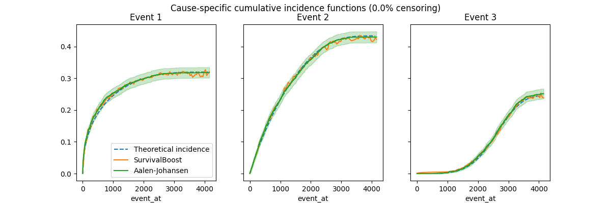
Here the data is generated by taking the minimum time of samples from three competing Weibull distributions with fixed parameters and without any conditioning covariate. In this case, the Aalen-Johansen estimator is expected to be unbiased, and this is empirically confirmed by this example.

The hazardous.SurvivalBoost estimator on the other hand is a predictive estimator that expects at least one conditioning covariate. In this example, we use a dummy covariate that is constant for all samples. Here we are not interested in the discrimination power of the estimator: there is none by construction, since we do not have access to informative covariates. Instead we empirically study its marginal calibration, that is, its ability to approximately recover an unbiased estimate of the marginal cumulative incidence function for each competing event.

This example also highlights that hazardous.SurvivalBoost estimates noisy cumulative incidence functions, which are not smooth and not even monotonically increasing. This is a known limitation of the estimator, and attempting to enforce monotonicity at training time typically introduces severe over-estimation bias for large time horizons.

from time import perf_counter
import numpy as np
import matplotlib.pyplot as plt

from hazardous import SurvivalBoost
from hazardous.data import make_synthetic_competing_weibull
from lifelines import AalenJohansenFitter

n_samples = 3_000
base_scale = 1_000.0  # some arbitrary time unit
event_dist_shapes = (0.5, 1.0, 5.0)
event_dist_scales = (10, 3, 3)
n_events = len(event_dist_shapes)

_, y_uncensored = make_synthetic_competing_weibull(
    n_samples=n_samples,
    n_events=n_events,
    censoring_relative_scale=0,
    return_X_y=True,
    shape_ranges=[(shape, shape) for shape in event_dist_shapes],
    scale_ranges=[(scale, scale) for scale in event_dist_scales],
    base_scale=base_scale,
    random_state=0,
)

t_max = y_uncensored["duration"].max()

Since we know the true distribution of the data, we can compute the theoretical cumulative incidence functions (CIFs) by integrating the hazard functions. The CIFs are the probability of experiencing the event of interest before time t, given that the subject has not experienced any other event before time t.

The following function computes the hazard function of a Weibull distribution:

def weibull_hazard(t, shape=1.0, scale=1.0):
    # Plug an arbitrary finite hazard value at t==0 because fractional powers
    # of 0 are undefined.
    #
    # XXX: this does not seem correct but in practice it does make it possible
    # to integrate the hazard function into cumulative incidence functions in a
    # way that matches the Aalen Johansen estimator.
    with np.errstate(divide="ignore"):
        return np.where(t == 0, 0.0, (shape / scale) * (t / scale) ** (shape - 1.0))

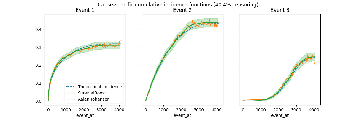
Note that true CIFs are independent of the censoring distribution. We can use them as reference to check that the estimators are unbiased by the censoring.

We first define the two estimators of interest. The hazardous.SurvivalBoost instance uses the Kaplan-Meier estimator on the negated event labels (1 for censoring, 0 for any event) to estimate internal IPCW weights. This is a valid choice in this context because we do not have access to any informative covariate (either for censoring or for the events of interest).

calculate_variance = n_samples <= 5_000
aj = AalenJohansenFitter(calculate_variance=calculate_variance, seed=0)

survival_boost = SurvivalBoost(
    learning_rate=0.03,
    n_iter=100,
    max_leaf_nodes=5,
    hard_zero_fraction=0.1,
    min_samples_leaf=50,
    show_progressbar=False,
    ipcw_strategy="kaplan-meier",
    random_state=0,
)

CIFs estimated on uncensored data

Let’s now estimate the CIFs on uncensored data and plot them against the theoretical CIFs:

def plot_cumulative_incidence_functions(y, survival_boost=None, aj=None):
    """Plot cause-specific cumulative incidence per event using a dummy covariate"""
    _, axes = plt.subplots(figsize=(12, 4), ncols=n_events, sharey=True)

    # Compute the estimate of the CIFs on a coarse grid.
    coarse_timegrid = np.linspace(0, t_max, num=100)

    # Compute the theoretical CIFs by integrating the hazard functions on a
    # fine-grained time grid. Note that integration errors can accumulate quite
    # quickly if the time grid's resolution is too coarse, especially for the
    # Weibull distribution with shape < 1.
    tic = perf_counter()
    fine_time_grid = np.linspace(0, t_max, num=10_000_000)
    dt = np.diff(fine_time_grid)[0]
    all_hazards = np.stack(
        [
            weibull_hazard(fine_time_grid, shape, scale * base_scale)
            for shape, scale in zip(event_dist_shapes, event_dist_scales)
        ],
        axis=0,
    )
    any_event_hazards = all_hazards.sum(axis=0)
    any_event_survival = np.exp(-(any_event_hazards.cumsum(axis=-1) * dt))
    print(
        "Integrated theoretical any event survival curve in"
        f" {perf_counter() - tic:.3f} s"
    )

    censoring_fraction = (y["event"] == 0).mean()
    plt.suptitle(
        "Cause-specific cumulative incidence functions"
        f" ({censoring_fraction:.1%} censoring)"
    )
    # Non-informative covariate because scikit-learn estimators expect at least
    # one feature.
    X_dummy = np.zeros(shape=(n_samples, 1), dtype=np.float32)
    if survival_boost is not None:
        tic = perf_counter()
        survival_boost.fit(X_dummy, y)
        duration = perf_counter() - tic
        print(f"SurvivalBoost fit: {duration:.3f} s")
        tic = perf_counter()
        cif_preds = survival_boost.predict_cumulative_incidence(
            X_dummy, coarse_timegrid
        )
        duration = perf_counter() - tic
        print(f"SurvivalBoost prediction: {duration:.3f} s")

    for event_id, (ax, hazards_i) in enumerate(zip(axes, all_hazards), 1):
        theoretical_cif = (hazards_i * any_event_survival).cumsum(axis=-1) * dt
        print(
            "Integrated theoretical cumulative incidence curve for event"
            f" {event_id} in {perf_counter() - tic:.3f} s"
        )
        downsampling_rate = fine_time_grid.size // coarse_timegrid.size
        ax.plot(
            fine_time_grid[::downsampling_rate],
            theoretical_cif[::downsampling_rate],
            linestyle="dashed",
            label="Theoretical incidence",
        ),

        if survival_boost is not None:
            cif_pred = cif_preds[:, event_id][0]
            ax.plot(
                coarse_timegrid,
                cif_pred,
                label="SurvivalBoost",
            )
            ax.set(title=f"Event {event_id}")

        if aj is not None:
            # Randomly break tied durations, to silence a warning raised by the
            # Aalen-Johansen estimator.
            rng = np.random.default_rng(0)
            jitter = rng.normal(scale=1e-3, size=y.shape[0])
            tic = perf_counter()
            aj.fit(y["duration"] + jitter, y["event"], event_of_interest=event_id)
            duration = perf_counter() - tic
            print(f"Aalen-Johansen for event {event_id} fit in {duration:.3f} s")
            aj.plot(label="Aalen-Johansen", ax=ax)

        if event_id == 1:
            ax.legend(loc="lower right")
        else:
            ax.legend().remove()


plot_cumulative_incidence_functions(
    survival_boost=survival_boost, aj=aj, y=y_uncensored
)

Integrated theoretical any event survival curve in 0.662 s
SurvivalBoost fit: 2.690 s
SurvivalBoost prediction: 2.927 s
Integrated theoretical cumulative incidence curve for event 1 in 2.988 s
Aalen-Johansen for event 1 fit in 4.937 s
Integrated theoretical cumulative incidence curve for event 2 in 5.032 s
Aalen-Johansen for event 2 fit in 5.018 s
Integrated theoretical cumulative incidence curve for event 3 in 5.096 s
Aalen-Johansen for event 3 fit in 4.976 s

CIFs estimated on censored data

Add some independent censoring with some arbitrary parameters to control the amount of censoring: lowering the expected value bound increases the amount of censoring.

_, y_censored = make_synthetic_competing_weibull(
    n_samples=n_samples,
    n_events=n_events,
    censoring_relative_scale=1.5,
    return_X_y=True,
    shape_ranges=[(shape, shape) for shape in event_dist_shapes],
    scale_ranges=[(scale, scale) for scale in event_dist_scales],
    base_scale=base_scale,
    random_state=0,
)

plot_cumulative_incidence_functions(survival_boost=survival_boost, aj=aj, y=y_censored)

Integrated theoretical any event survival curve in 0.591 s
SurvivalBoost fit: 2.705 s
SurvivalBoost prediction: 2.940 s
Integrated theoretical cumulative incidence curve for event 1 in 3.000 s
Aalen-Johansen for event 1 fit in 4.967 s
Integrated theoretical cumulative incidence curve for event 2 in 5.058 s
Aalen-Johansen for event 2 fit in 4.967 s
Integrated theoretical cumulative incidence curve for event 3 in 5.045 s
Aalen-Johansen for event 3 fit in 5.035 s

Note that the Aalen-Johansen estimator is unbiased and empirically recovers the theoretical curves both with and without censoring. The SurvivalBoost estimator also appears unbiased by censoring, but the predicted curves are not smooth and not even monotonically increasing. By adjusting the hyper-parameters, notably the learning rate, the number of boosting iterations and leaf nodes, it is possible to somewhat control the smoothness of the predicted curves, but it is likely that doing some kind of smoothing post-processing could be beneficial (but maybe at the cost of introducing some bias). This is left as future work.

Alternatively, we could try to enable a monotonicity constraint at training time, however, in practice this often causes a sever over-estimation bias for the large time horizons: